Complete Guide to Pivot Tables in Excel for Mac
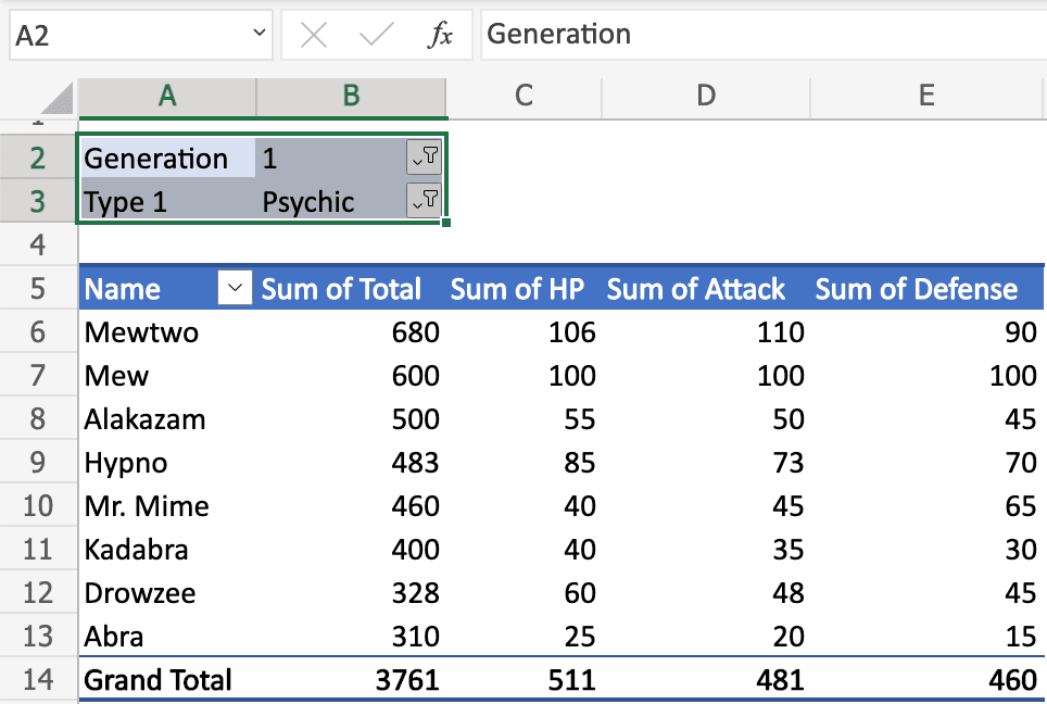
Quick Answer: Select your data, then go to Insert > PivotTable. There is no default single-key shortcut for inserting a PivotTable on Mac (confirm exact key combo) — most users use the Ribbon or menu. Once created, drag fields into Rows, Columns, Values, and Filters to summarize thousands of rows into a readable table in seconds. Mac Excel Shortcuts app also remaps your old Windows PivotTable ribbon-navigation shortcuts so you're not relearning the menu from scratch.
User problem
You've got a spreadsheet with hundreds or thousands of rows — sales transactions, survey responses, expense line items — and you need answers fast: total revenue by region, average order size by month, headcount by department. Scrolling and manually summing is slow and error-prone. On Windows, you probably built PivotTables with Alt N V or a familiar toolbar button. On Mac, the menus have moved, some keyboard shortcuts don't exist, and the PivotTable Fields pane looks and behaves slightly differently. This guide gets you from raw data to a working PivotTable, the Mac way.
What the feature does
A PivotTable takes flat, row-based data and lets you dynamically summarize it — grouping, counting, summing, and averaging — without writing a single formula. You drag column headers ("fields") into four buckets: Rows, Columns, Values, and Filters. Excel recalculates the summary instantly whenever you rearrange fields or the underlying data changes (after a refresh).
When to use it
You need a summary (sum, count, average, min/max) broken down by one or more categories.
Your raw data has repeated categorical values (e.g., "Region," "Product," "Month") that you want to group by.
You want to slice the same dataset multiple ways without duplicating formulas.
You're building a recurring report and want a reusable, refreshable structure.
Prerequisites
Your data should be in a proper table format: one header row, no blank rows or merged cells, and each column consistently typed (text, number, or date).
Ideally, convert your range to an Excel Table first (Insert > Table, or Command-T) — this makes the PivotTable auto-expand when you add new rows later.
Method 1: Ribbon
Click anywhere inside your data range.
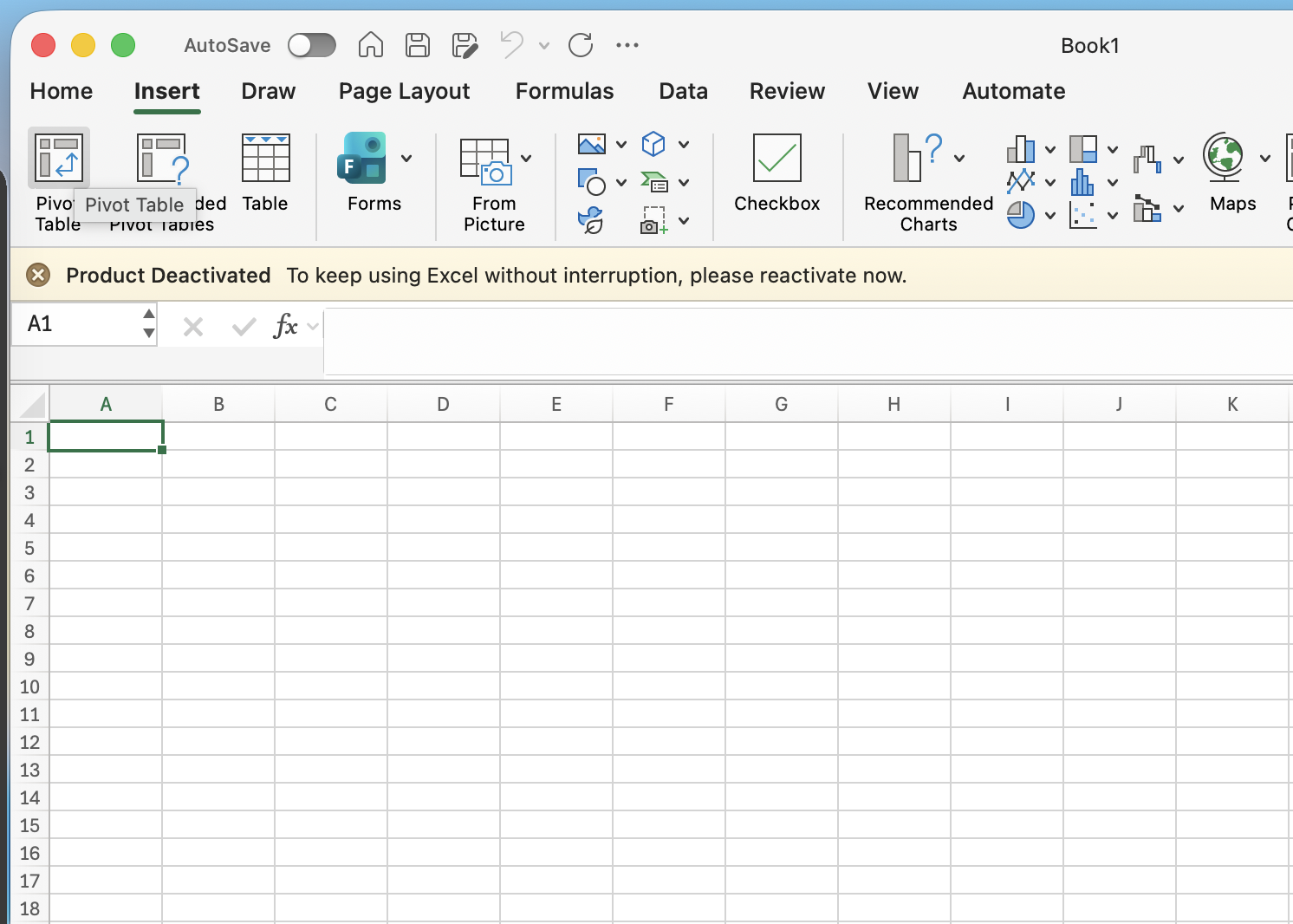
Go to the Insert tab on the Ribbon.
Click PivotTable (it's usually one of the first icons, on the left side of the Insert tab).
In the dialog, confirm the data range is correct and choose New Worksheet (recommended for beginners) or Existing Worksheet.
Click OK. A blank PivotTable and the PivotTable Fields pane appear on the right.
Method 2: Menus
If you prefer the classic menu bar (or the Ribbon is hidden): Insert > PivotTable... from the top menu bar works identically to the Ribbon button and opens the same dialog. This is useful if you've collapsed the Ribbon to get more screen space, which is common on smaller MacBook displays.
Method 3: Native keyboard shortcuts
Mac Excel does not ship a default keyboard shortcut to insert a PivotTable — this is one of the more jarring gaps for Windows migrators who relied on Alt N V. There is no direct Mac equivalent because Mac Excel's Ribbon doesn't support the same Alt-key "KeyTip" navigation system Windows Excel uses.
Once your PivotTable exists, these shortcuts help you work faster:
Refresh all data connections: Command-Option-F5. For a single PivotTable, right-click inside it and choose Refresh, or use Data > Refresh All. (confirm exact key combo for single-pivot refresh)
Group selected items: Shift-Option-Right Arrow (mirrors the Windows Shift+Alt+Right Arrow for grouping dates or numbers).
Ungroup: Shift-Option-Left Arrow.
Move between field pane sections: Tab cycles focus through the PivotTable Fields pane once it has focus.
You can create a custom shortcut yourself via Tools > Customize Keyboard... in Excel's menu bar, which lets you assign a key combination to the "InsertPivotTable" command if you build PivotTables often enough to justify it.
Method 4: Mouse workflow
Click and drag to select your data range (or click one cell inside a Table and let Excel auto-detect the range).
In the PivotTable Fields pane, drag a categorical field (like "Region") into the Rows box.
Drag a numeric field (like "Revenue") into the Values box — Excel defaults to Sum for numbers and Count for text.
Drag another categorical field (like "Product Category") into Columns to create a cross-tab.
Drag a field into Filters to add a dropdown that lets viewers slice the whole table (e.g., filter by fiscal year).
Right-click any value cell to change the summary type — Sum, Average, Count, Max, Min, or a custom calculation.
Method 5: Maccove workflow
If you built PivotTables constantly on Windows using Alt N V and other keyboard chains, Mac Excel Shortcuts app lets you keep using your old Windows shortcut muscle memory directly — it remaps familiar Windows Excel key sequences to their closest Mac Excel action, so you don't have to relearn a new set of commands mid-project. It won't invent shortcuts Mac Excel doesn't support (like a native PivotTable insert key), but it smooths over dozens of smaller friction points around navigating the Ribbon and menus.
Real-world example
Say you have a CSV export from your CRM with columns: Date, Sales Rep, Region, Product, Units Sold, Revenue. You want total revenue by Region and by Product.
Select the data, Insert > PivotTable, OK.
Drag Region to Rows, Product to Columns, Revenue to Values.
Right-click a value, confirm it's set to Sum, not Count.
Drag Date to Filters, then filter to the current quarter.
You now have a live cross-tab of revenue by region and product, filterable by quarter, that updates whenever you refresh the underlying data.
Common mistakes
Blank rows or columns in the source data — Excel will silently truncate the detected range. Always check the range in the Create PivotTable dialog.
Merged cells in headers — these break field detection. Unmerge before building the PivotTable.
Forgetting to refresh — editing source data does not auto-update the PivotTable. Right-click and choose Refresh, or use Data > Refresh All.
Summing text-like numbers — if numbers are stored as text (common in CSV imports), Excel will Count instead of Sum. Convert the column to Number format first.
Windows equivalent
On Windows, Alt N V opens the Create PivotTable dialog directly via KeyTips. Mac Excel's Ribbon doesn't support KeyTip letter-navigation, so this exact shortcut has no Mac equivalent — you'll use the mouse or a custom-assigned shortcut instead. Field-dragging behavior, Values/Rows/Columns/Filters terminology, and grouping options are otherwise nearly identical between platforms.
FAQs
Can I create a PivotTable from data in another workbook?
Yes — when creating the PivotTable, choose an external range, or better, use Power Query to import and combine data first.
Why does my PivotTable show "Count" instead of "Sum" for a numeric column?
The source column likely contains text-formatted numbers or blank cells. Check for a small green triangle in the cell corner indicating text-stored numbers.
Can I have multiple PivotTables from the same source data?
Yes, and it's efficient to do so — right-click an existing PivotTable's data source and choose to base a new one on the same pivot cache to avoid duplicating memory usage.