How Do You Create an Interactive Dashboard in Excel on Mac?
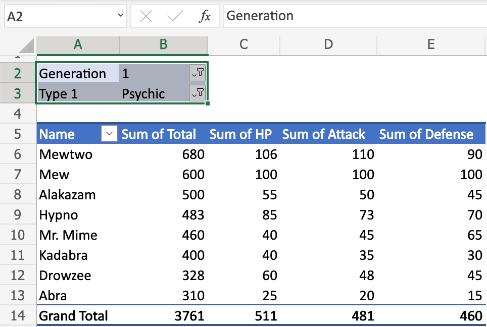
Quick Answer: Build one or more PivotTables/PivotCharts from clean source data, add Slicers (Insert > Slicer) so viewers can filter by category without touching formulas, arrange everything on a dedicated Dashboard tab, and hide gridlines/row-column headers for a polished, presentation-ready look — all achievable natively in Excel for Mac without add-ins. Mac Excel Shortcuts app keeps your copy/paste and navigation shortcuts consistent while you build this, and adds a shortcut for Remove Duplicates during the data-prep step.
Goal & sample dataset
A dashboard turns a static report into something a manager can explore themselves — click a Region filter and every chart updates. This is fully supported on Mac, though the interface for building Slicers differs slightly from Windows.
Sample dataset: the same sales dataset from the Monthly Report workflow — Date, Sales Rep, Region, Product, Units, Revenue — around 2,000 rows.
Estimated time
60–90 minutes for a first build with 3–4 visuals and 2 slicers. Rebuilding for a new dataset: 20 minutes.
Skills required
PivotTables
Basic charting
Comfort with cell/object alignment for a clean visual layout
Step-by-step solution
Step 1: Prepare source data and a hidden "Data" tab
Clean and Table-ify your source data. Keep this on a tab named Data, which you'll hide once the dashboard is built.
Step 2: Build the underlying PivotTables
Build 2–3 PivotTables on a working tab: Revenue by Region, Revenue by Month, Units by Product.
Step 3: Turn PivotTables into PivotCharts
Click inside a PivotTable.
Insert > PivotChart.
Repeat for each PivotTable you want visualized.
Step 4: Add Slicers for interactive filtering
Click any PivotTable.
Insert > Slicer.
Check the fields you want as filters — typically Region and Product.
By default, a Slicer only filters the PivotTable it was inserted from. To connect one Slicer to all PivotCharts: click the Slicer, go to Report Connections, check every PivotTable that should respond.
Step 5: Assemble the Dashboard tab
Insert a new tab named Dashboard, cut each PivotChart and Slicer from the Pivots tab, and paste them onto it (Command-X, click Dashboard, Command-V).
Step 6: Polish the visual presentation
Uncheck Gridlines and Headings under View, set a light background fill, and add a title text box.
Step 7: Test the interactivity
Click through each Slicer and confirm every connected chart updates simultaneously.
Faster keyboard-only workflow
Dashboard building is inherently visual and mouse-heavy, but you can speed up the data/pivot phase:
Command-T to Table-ify source data.
Command-Option-F5 to refresh all PivotTables/charts.
Tab / Shift-Tab to cycle between inserted objects.
Productivity tips
Build your dashboard on a copy of the workbook first.
Use consistent color coding across charts.
Slicer styling and Report Connections are two areas where the Mac Ribbon layout differs most from Windows — Mac Excel Shortcuts app lets you use your old Windows shortcut muscle memory directly for surrounding tasks like copy/paste and navigation.
FAQs
Can I use Slicers with regular Tables, not just PivotTables?
Yes — since Excel 2013/Mac Excel 2016+, Slicers work on regular Excel Tables too.
Can I share this dashboard with someone who doesn't have Excel?
Export a static snapshot via File > Export > Create PDF, or they'll need Excel to interact with filters.